Using RMarkdown

Overview

Teaching: 10 min
Exercises: 2 min

Questions

• How do I write a lesson using RMarkdown?

Objectives

• Explain how to use RMarkdown with the new lesson template.

• Demonstrate how to include pieces of code, figures, and challenges.

This episode demonstrates all the features that can be used when writing a lesson in RMarkdown.

When rendering a lesson written in RMarkdown, the lesson template does two things:

1. It identifies the dependencies (the R packages) that your lesson uses and installs them in your library.
2. It converts the RMarkdown files (the files in the .Rmd extension in the _episodes_rmd folder) into Markdown files in the _episodes folder.

Depending on whether it uses the remote theme (most lessons in the Carpentries Incubator, and most R-based Data Carpentry lessons) or the theme from the styles repository, the details of how the site is created differ. In practice, little changes for you unless you want to host a functioning version of the site as a fork. The section “Hosting a fork” below provides more information.

Structure of a RMarkdown file in the _episodes_rmd folder

Our template requires that the YAML header of your RMarkdown file includes the source: Rmd in addition of the other entries that are expected. For instance, the YAML header for this episode is:

---
source: Rmd
title: "Using RMarkdown"
teaching: 10
exercises: 2
questions:
- "How to write a lesson using RMarkdown?"
objectives:
- "Explain how to use RMarkdown with the new lesson template."
- "Demonstrate how to include pieces of code, figures, and challenges."
keypoints:
- "Edit the .Rmd files not the .md files"
- "Run `make serve` to knit documents and preview lesson website locally"
---

RMarkdown episode files should include an extra source field in the page front matter, telling the lesson template to point to the RMarkdown file in the source repository, instead of the knitted Markdown equivalent:

---
source: Rmd
title: Episode Title
[...]

Every episode written in RMarkdown must include the block below at the beginning of the page body i.e. after the page front matter.

```{r, include=FALSE}
source("../bin/chunk-options.R")
knitr_fig_path("05-")
```

The first line ensures that the chunks have the correct styling in the rendered website. The second line is optional but allows you to ensure that figures that are generated by the lessons will have the same prefix for each episode (you should use a different prefix for each episode using the episode number for instance).

The rest of the lesson should be written as a normal RMarkdown file. You can include chunks for codes, just like you would normally do. Output of code chunks will be generated as part of the knitting process.

Normal output:

```{r}
1 + 1
```

will be rendered as

1 + 1

[1] 2

Output with error message:

```{r}
x[10]
```

will be rendered as

x[10]

Error in eval(expr, envir, enclos): object 'x' not found

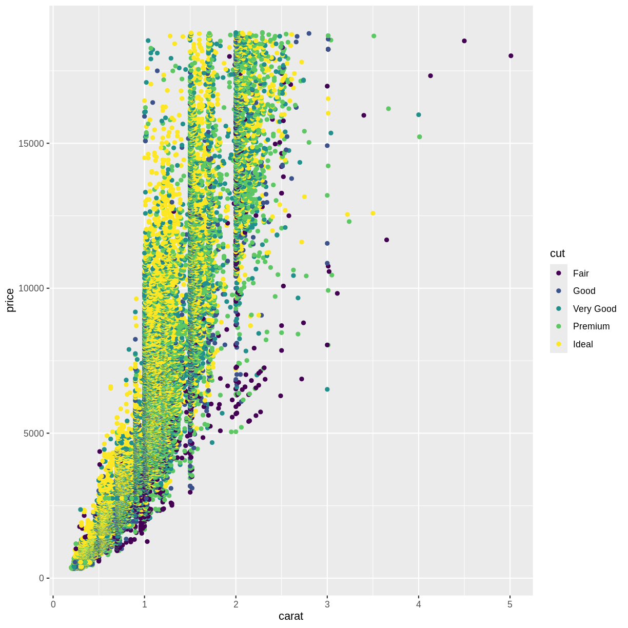
Similarly, any figures generated by code chunks will be embedded below the chunk in the page:

```{r plot-example, fig.cap="An example figure plotting carat of diamonds against their price, with the colour of the data points based on the cut of the diamond."}
library(ggplot2)
ggplot(diamonds, aes(x = carat,  y = price, color = cut)) +
    geom_point()
```

will be rendered as

library(ggplot2)
ggplot(diamonds, aes(x = carat,  y = price, color = cut)) +
    geom_point()

The alternative text for these embedded images will be the same as the figure caption specified with the fig.cap parameter. If you would like the value of the figure’s alternative text to be different to its caption, you can specify the fig.alt parameter on the code chunk too. If you do not specify fig.cap or fig.alt, the figure will be given generic alternative text, which may reduce the accessibility of your lesson e.g. by providing less information to learners using screen readers.

For the challenges and their solutions, you need to pay attention to where the > go and where to leave blank lines. You can include code chunks in both the instructions and solutions. For instance this:

> ## Challenge: Can you do it?
>
> What is the output of this command?
>
> ```{r, eval=FALSE}
> paste("This", "new", "template", "looks", "good")
> ```
>
> > ## Solution
> >
> > ```{r, echo=FALSE}
> > paste("This", "new", "template", "looks", "good")
> > ```
> {: .solution}
{: .challenge}

will generate this:

Challenge: Can you do it?

What is the output of this command?

paste("This", "new", "template", "looks", "good")

Solution

[1] "This new template looks good"

On Branch Names and Automation

For lessons that do not use R, the code included in the lessons is not evaluated. Each time a new commit is pushed to the repository, GitHub can take these files and directly render their content using Jekyll to create the lesson website. Because it is a one-step process, we can use the same branch (gh-pages) to develop the lesson and render its content as a website. However, for R-based lessons, we first need to convert the RMarkdown to Markdown, and then, we need to instruct GitHub to generate the lesson website from the rendered Markdown files. Because of this two-step process, we use two branches: one is used to develop the content of the lesson (typically main) and the other is only used to host the files that will generate the lesson website (gh-pages). To automatically convert the files from RMarkdown to Markdown, and push these Markdown files to GitHub, we rely on a GitHub Actions workflow (typically in the .github/workflows/website.yml file in the lesson repository).

Key Points

• Edit the .Rmd files not the .md files

• Run make serve to knit documents and preview lesson website locally