All in One View
Content from Introduction to The Carpentries Workbench
Last updated on 2026-05-26 | Edit this page
Estimated time: 12 minutes
Overview
Questions
- How do I get started?
Objectives
- Create new lesson from scratch
- Identify the main command to preview the site
- Understand the basic structure of a new workbench
Let’s say you have a set of Markdown or R Markdown files that you used for a class website that you want to convert into a Carpentries Lesson. To go from zero to a new lesson website that can auto-render R Markdown documents to a functional website is three steps with sandpaper:
- Create a site
- Push to GitHub
- Add your files
That’s it. After that, if you know how to write in Markdown, you are good to go.
Takeaway message
Contributors should only be expected to know basic markdown and very minimal yaml syntax in order to work on lessons.
Super Quickstart: Copy A Template from GitHub
The absolute quickest way to get started with The Carpentries Workbench is to create a GitHub repository with one of the two available templates, depending on your preference:
Step 1: Choose a template
- Markdown Lessons (no generated content) (if your lesson will not include R code examples, use this template)
- R Markdown Lessons (generated content via R) (our tutorial uses this template)
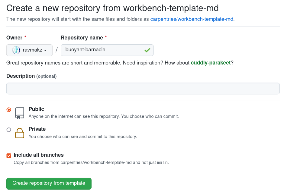
Step 2: Choose a name for your lesson repository.
Name it “buoyant-barnacle”. select “Include All Branches”. Click on the button that says “Create repository from template”
Creating a new lesson repository
Step 3: Customise your site
On GitHub, open the config.yaml file, and click on the
pencil icon on the top and edit the values, especially “carpentry”,
“source”, and “title” to reflect your own repository. Commit the file
using the form at the bottom of the page.
That’s it. The website should update in about 2-3 minutes with your information. If you want to continue working directly on GitHub, you can do so. If you want to work locally, be sure to follow the setup instructions, clone your lesson to your computer, open RStudio (or your preferrred interface to R) inside the lesson folder, and preview your new lesson
Quickstart: Create a New Lesson
Create a Lesson Locally
Follow these steps to create a brand new lesson on your Desktop called “buoyant-barnacle”.
- Follow the setup instructions
- Open RStudio (or your preferred interface to R)
- Use the following code:
R
library("fs") # file system package for cross-platform paths
library("sandpaper")

# Create a brand new lesson on your desktop called "buoyant-barnacle"
bb <- path_home("Desktop/buoyant-barnacle")
print(bb) # print the new path to your screen
create_lesson(bb) # create a new lesson in that path
If everything went correctly, you will now have a new RStudio window
open to your new project called “buoyant-barnacle” on your Desktop (if
you did not use RStudio, your working directory should have changed, you
can check it via the getwd() command).
Your lesson will be initialized with a brand new git repository with
the initial commit message being
Initial commit [via {sandpaper}].
🪲 Known Quirk
If you are using RStudio, then an RStudio project file
(*.Rproj) is automatically created to help anchor your
project. You might notice changes to this file at first as RStudio
applies your global user settings to the file. This is perfectly normal
and we will fix this in a future iteration of {sandpaper}.
Previewing Your New Lesson
After you created your lesson, you will want to preview it locally. First, make sure that you are in your newly-created repository and then use the following command:
R
sandpaper::serve()
What’s with the :: syntax?
This is a syntax that clearly states what package a particular
function comes from. In this case, sandpaper::serve() tells
R to use the serve() function from the
sandpaper package. These commands can be run without first
calling library(<packagename>), so they are more
portable. I will be using this syntax for the rest of the lesson.
If you are working in RStudio, you will see a preview of your lesson in the viewer pane and if you are working in a different program, a browser window will open, showing a live preview of the lesson. When you edit files, they will automatically be rebuilt to your website.
DID YOU KNOW? Keyboard Shortcuts are Available
If you are using RStudio, did you know you can use keyboard shortcuts to render the lesson as you are working on the episodes?
- Render and preview the whole lesson
- ctrl + shift + B
- Render and preview an episode
- ctrl + shift + K
The first time you run this function, you might see A LOT of output on your screen and then your browser will open the preview. If you run the command again, you will see much less output. If you like to would like to know how everything works under the hood, you can check out the {sandpaper} package documentation.
How do I determine the order of files displayed on the website?
The config.yaml file contains four fields that
correspond to the folders in your repository: episodes,
instructors, learners, profiles.
If the list is empty, then the files in the folders are displayed in
alphabetical order, but if you want to customize exactly what content is
published on the website, you can add a yaml list of the filenames to
determine order.
For example, if you had three episodes called “introduction.md”,
“part_two.Rmd”, and “in_progress.md” and you wanted to only show
introduction and part_two, you would edit config.yaml to
list those two files under episodes::
Push to GitHub
The lesson you just created lives local on your computer, but still needs to go to GitHub. At this point, we assume that you have successfully linked your computer to GitHub.
- visit https://github.com/new/
- enter
buoyant-barnacleas the repository name - Press the green “Create Repository” button at the bottom of the page
- Follow the instructions on the page to push an existing repository from the command line.
A few minutes after you pushed your repository, the GitHub workflows
would have validated your lesson and created deployment branches. You
can track the progress at
https://github.com/<USERNAME>/buoyant-barnacle/actions/.
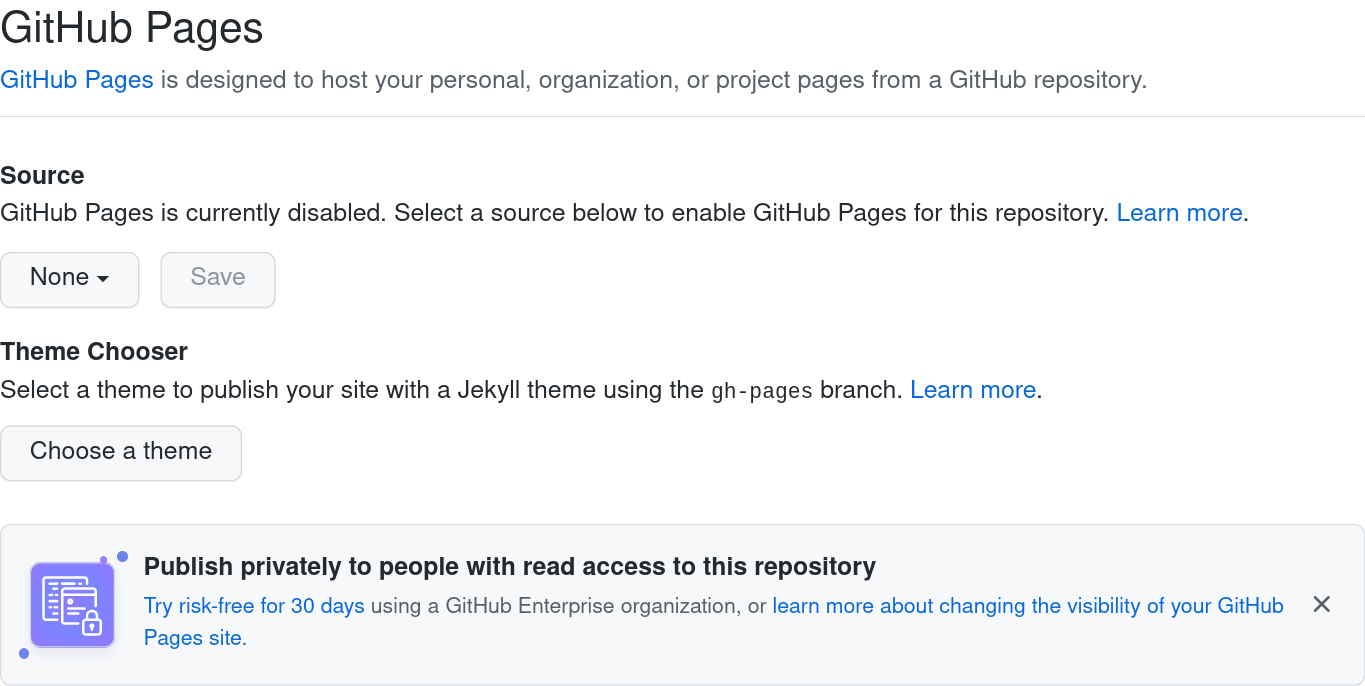
Once you have a green check mark, you can set
up GitHub Pages by going to
https://github.com/<USERNAME>/buoyant-barnacle/settings/pages
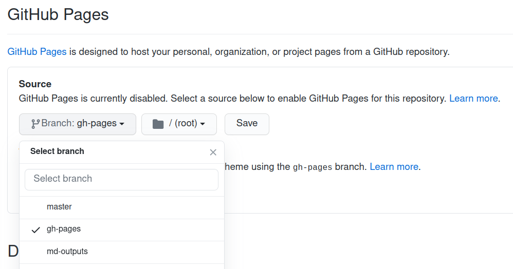
and choosing gh-pages from the dropdown menu as shown in
the image below:
Click on the “select branch” button and select “gh-pages”, then click “Save”:
After completing this configuration, the URL for your lesson website
will be displayed at the top of the page. Site URLs can be customised,
but the default URL structure is
https://<USERNAME>.github.io/<REPONAME>/: the
URL of the buoyant-barnacle example used so far would be
https://<USERNAME>.github.io/buoyant-barnacle/.
⌛ Be Patient
GitHub needs to start up a new virtual machine the first time you use this, so it may take anywhere from 4 minutes up to 30 minutes for things to get started: 15 minutes for the workflow to spin up and then another 15 minutes for the machine to bootstrap and cache.
Alternative: Two-step solution in R
If you use R and use an HTTPS protocol, this can be done in a single step from inside RStudio with the {usethis} package:
R
usethis::use_github()
usethis::use_github_pages()
The use_github() function will set up a new repository
under your personal account called buoyant-barnacle, add
that remote to your git remotes, and automatically push
your repository to GitHub.
The use_github_pages() function will signal to GitHub
that it should allow the gh-pages branch to serve the
website at https://user.github.io/buoyant-barnacle
The output of these commands should look something like this:
OUTPUT
> use_github()
✔ Creating GitHub repository 'zkamvar/buoyant-barnacle'
✔ Setting remote 'origin' to 'https://github.com/zkamvar/buoyant-barnacle.git'
✔ Pushing 'main' branch to GitHub and setting 'origin/main' as upstream branch
✔ Opening URL 'https://github.com/zkamvar/buoyant-barnacle'

> use_github_pages()
✔ Initializing empty, orphan 'gh-pages' branch in GitHub repo 'zkamvar/buoyant-barnacle'
✔ GitHub Pages is publishing from:
• URL: 'https://zkamvar.github.io/buoyant-barnacle/'
• Branch: 'gh-pages'
• Path: '/'
If you don’t use the HTTPS protocol, and want to find out how to set it in R, we have a walkthrough to set your credentials in the learners section.
Tools
As described in the setup document, The Carpentries Workbench only requires R and pandoc to be installed. The tooling from the styles lesson template has been split up into three R packages:
- {varnish} contains the HTML, CSS, and JavaScript elements
- {pegboard} is a validator for the markdown documents
- {sandpaper} is the engine that puts everything together.
- Lessons can be created with
create_lesson() - Preview lessons with
serve() - The toolchain is designed to be modular.
Content from Episode Structure
Last updated on 2026-05-26 | Edit this page
Estimated time: 17 minutes
Overview
Questions
- How do you create a new episode?
- What syntax do you need to know to contribute to a lesson with The Carpentries Workbench?
- How do you write challenge blocks?
- What syntax do you use to write links?
- How do you include images?
- How do you include math?
- How do you include Glosario terms?
Objectives
- Practise creating a new episode with R
- Understand the required elements for each episode
- Understand pandoc-flavored markdown
- Demonstrate how to include pieces of code, figures, and nested challenge blocks
Introduction
An episode1 is an individual unit of a lesson that focuses on a single topic with clear questions, objectives, and key points. If a lesson goal is to teach you about using git, an individual episode would teach you how to inspect the status of a git repsitory. The idea behind the name “episode” is the thought that each one should last about as long as an episode for an television series.
As we will cover in the next episode, all
of the episodes live inside the episodes/ directory at the
top of the lesson folder. Their order is dictated by the
episodes: element in the config.yaml file (but
defaults to alphabetical). The other folders (learners/,
instructors/, and profiles/) are similarly
configured. This episode will briefly explain how to edit markdown
content in the lessons.
Buoyant Barnacle
The exercises in this episode correspond to the Buoyant Barnacle repository you created in the Introduction
There are three things you should be comfortable with in order to contribute to a lesson 2
- Writing basic and extended markdown syntax
- Writing Fenced div elements to create callouts and exercise blocks
- Writing simple yaml lists
Creating A New Episode
To create a new episode, you should open your lesson
(buoyant-barnacle) in your RStudio or your favorite text
editor and in the R console type:
R
sandpaper::create_episode("next-episode")
This will create a new episode in the episodes folder called
“02-next-episode.Rmd”. If you already have your episode schedule set in
config.yaml, then this episode will not be rendered in the
site and will remain a draft until you add it to the schedule. Next, we
will show how you can add a title and other elements to your
episode.
What is the .Rmd extension?
You might notice that the new episode has the extension of
.Rmd instead of .md. This is R Markdown, an
extension of markdown that allows us to insert special code fences that
can execute R code and automatically produce output chunks with controls
of how the output and input are rendered in the document.
For example, this markdown code fence will not produce any output, but it is valid for both Markdown and R Markdown.
R
print("hello world!")
But when I open the fence with ```{r} then it becomes an
R Markdown code fence and will execute the code inside the fence:
R
print("hello world!")
OUTPUT
[1] "hello world!"Note that it is completely optional to use these special code fences!
Required Elements
To keep with our active learning principles, we want to be mindful about the content we present to the learners. We need to give them a clear title, questions and objectives, and an estimate of how long it will take to navigate the episode (though this latter point has shown to be demoralizing). Finally, at the end of the episode, we should reinforce the learners’ progress with a summary of key points.
YAML metadata
The YAML syntax of an episode contains three elements of metadata associated with the episode at the very top of the file:
YAML
---
title: "Using RMarkdown For Automated Reports" # Episode title
teaching: 5   # teaching time in minutes
exercises: 10 # exercise time in minutes
---

## First Episode SectionCreate a Title
Your new episode needs a title!
- Open the new episode in your editor
- edit the title
- add the episode to the
config.yaml - preview it with
sandpaper::build_lesson()or using the ctrl + shift + k keyboard shortcut.
Did the new title show up?
Questions, Objectives, Keypoints
These are three blocks that live at the top and bottom of the episodes.
-
questionsare displayed at the beginning of the episode to prime the learner for the content -
objectivesare the learning objectives for an episode and are displayed along with the questions -
keypointsare displayed at the end of the episode to reinforce the objectives
They are formatted as pandoc fenced divisions, which we will explain in the next section:
Optional Elements
Lessons do not have to contain the following structural elements, but they can be useful for highlighting particular content.
Callout blocks
One of the key elements of our lessons are our callout blocks that give learners and instructors a bold visual cue to stop and consider a caveat or exercise. To create these blocks, we use pandoc fenced divisions, aka ‘fenced-divs’, which are colon-delimited sections similar to code fences that can instruct the markdown interpreter how the content should be styled.
Callout Component Guide
You can find a catalogue of the different callout blocks The Workbench supports in The Workbench Component Guide.
For example, to create a callout block, we would use
a blank line and at least three colons followed by the
callout tag (the tag designates an open fence), add our
content after a new line, and then close the fence with at least
three colons and no tag (which designates a closed fence):
This is a callout block. It contains at least three colons
However, it may be difficult sometimes to keep track of a section if it’s only delimited by three colons. Because the specification for fenced-divs require at least three colons, it’s possible to include more to really differentiate between these and headers or code fences:
MARKDOWN
::::::::::::::::::::::::::::::::::::::::::::::: testimonial

I'm **really excited** for the _new template_ when it arrives :grin:.

--- Toby Hodges

:::::::::::::::::::::::::::::::::::::::::::::::::::::::::::I’m really excited for the new template when it arrives 😁.
— Toby Hodges
Even better, you do not have to worry about counting colons! It doesn’t matter how many colons you put for the opening and closing fences, all that matters is you can visually see that the fences match.
That’s right, we can use emojis in The Carpentries Workbench! 💯 🎉
Tabbed content
Available from varnish v1.0.2, tabs are a great way to present
multiple pieces of information in a compact and organised way. You can
create them in two ways: firstly with a tab fenced div, and
secondly with a group-tab fenced div.
Whilst they both show content in the same way, grouped tabs differ from standard tabs in that they remember which tab you have selected across page changes. This can be useful if you want to use a specific tab throughout the lesson content, e.g. for a set of exercises or a set of solutions you want to use the “Windows” tab that was initially selected in the Setup episode.
The first tab specified is the default tab.
In both cases, tabs can hold callouts themselves and be specified within callouts too!
Tab
To create a tab group, create a tab fenced div, and then
add a level 3 markdown heading (###) for each tab you want
to create:
MARKDOWN
::: tab

### Windows

Some Windows instructions

### Mac

Maybe some for Mac

### Linux

And more for Linux users, including a code block:

```python
  print("Yay, tabs!")
```

:::Grouped tabs
Much like standard tabs, to create grouped tabs use a
group-tab fenced div, and then add a level 3 markdown
heading (###) for each tab you want to create:
MARKDOWN
::: group-tab

### Windows

1

### Mac

2

### Linux

3

:::

::: group-tab

### Windows

4

### Mac

5

### Linux

6

:::
The first tab specified is the default tab.
In the example below, selecting a tab in one tab group changes the tab in the other group(s).
(Thanks to @astroDimitrios for this great feature!)
Instructor Notes
The Carpentries Workbench supports separate instructor/learner views,
which allows for instructor notes to be incorporated into the lesson.
The default view of a lesson is the learner view, but you can switch to
the instructor view by scrolling to the top of the lesson, clicking on
the “Learner View” button at the top right, and then selecting
“Instructor View” from the dropdown. You can also add
instructor/ after the lesson URL (e.g. in this lesson, the
URL is
https://carpentries.github.io/sandpaper-docs/episodes.html;
to switch to the instructor view manually, you can use
https://carpentries.github.io/sandpaper-docs/instructor/episodes.html).
View the instructor note
When you visit this page, the default is learner view. Scroll to the top of the page and select “Instructor View” from the dropdown and return to this section to find an instructor note waiting for you.
MARKDOWN
::::::::::::::::::::::::::::::::::::: instructor
This is an instructor note. It contains information that can be useful for
instructors to know such as
- **Useful hints** about places that need extra attention
- **setup instructions** for live coding
- **reminders** of what the learners should already know
- anything else
```markdown
You can also include _any markdown elements_ like `code blocks`
```
{alt='a random image of a cute kitten'}
:::::::::::::::::::::::::::::::::::::::::::::::::This is an instructor note. It contains information that can be useful for instructors to know such as
- Useful hints about places that need extra attention
- setup instructions for live coding
- reminders of what the learners should already know
- anything else
Exercises/Challenges
The method of creating callout blocks with fences can help us create solution blocks nested within challenge blocks. Much like a toast sandwich, we can layer blocks inside blocks by adding more layers. For example, here’s how I would create a single challenge and a single solution:
MARKDOWN
::::::::::::::::::::::::::::::::::::: challenge

## Chemistry Joke

Q: If you aren't part of the solution, then what are you?

:::::::::::::::: solution

A: part of the precipitate

:::::::::::::::::::::::::
:::::::::::::::::::::::::::::::::::::::::::::::Chemistry Joke
Q: If you aren’t part of the solution, then what are you?
A: part of the precipitate
To add more content to the challenge, you close the first solution and add more text:
Challenge 1: Can you do it?
What is the output of this command?
R
paste("This", "new", "template", "looks", "good")
OUTPUT
[1] "This new template looks good"Challenge 2: how do you nest solutions within challenge blocks?
You can add a line with at least three colons and a
solution tag.
Now, here’s a real challenge for you
Yes! It is a valid fenced div for the following reasons:
- The opening fence has ≥3 colons
- The opening fence has a class designation
- The closing fence is on its own line and has ≥3 colons
Use Spoilers Instead of Floating Solution Blocks
When not attached to a challenge div, a formatted
solution block will be displayed with too much “buoyancy”
i.e. floating too high and obscuring some of the preceding content.
To avoid this, use the spoiler class of fenced div for
expandable/collapsible blocks of details instead of a floating
solution.
Expandable “Spoiler” Blocks
It can be helpful to provide “accordion” blocks of content that can be expanded and collapsed with a mouse click in some circumstances e.g. to provide detailed instructions for different operating systems, which can be examined by users based on their own system setup.
Such blocks of content can be added to a page with the
spoiler class of fenced div:
MARKDOWN
:::::::::::::::::::::::::::::::::::::::::: spoiler

### What Else Might We Use A Spoiler For?

- including a collapsed version of a very long block of output/a large image from a code block,
  which the learner can expand if they want to check their output against the lesson
- a reminder of some important concept/information required to follow the lesson,
  that you expect only some learners will need to read
- wrapping a set of optional exercises for an episode

::::::::::::::::::::::::::::::::::::::::::::::::::- including a collapsed version of a very long block of output/a large image from a code block, which the learner can expand if they want to check their output against the lesson
- a reminder of some important concept/information required to follow the lesson, that you expect only some learners will need to read
- wrapping a set of optional exercises for an episode
Code Blocks with Syntax Highlighting
To include code examples in your lesson, you can wrap it in three backticks like so:
Input:
Output:
thing = "python"
print("this is a {} code block".format(thing))
To include a label and syntax highlighting, you can add a label after the first set of backticks:
Input:
Output:
To indicate that a code block is an output block, you can use the label “output”:
Input:
MARKDOWN
```python
thing = "python"
print("this is a {} code block".format(thing))
```
```output
this is a python code block
```Output:
OUTPUT
this is a python code blockThe number of available languages for syntax highlighting are numerous and chances are, if you want to highlight a particular language, you can add the language name as a label and it will work. A full list of supported languages is here, each language being a separate XML file definition.
Tables
Tables in The Workbench follow the rules for pandoc pipe table syntax, which is the most portable form of tables.
Because we use pandoc for rendering, tables also have the following features:
- You can add a table caption, which is great for accessibility3
- You have control over the relative width of oversized table contents
Here is an example of a narrow table with three columns aligned left, center, and right, respectively.
MARKDOWN
Table: Four fruits with color and price in imaginary dollars

| fruit     | color                | price    |
| ------    | :--------------:     | -------: |
| apple     | :red_circle:         | \$2.05   |
| pear      | :green_circle:       | \$1.37   |
| orange    | :orange_circle:      | \$3.09   |
| gum gum fruit | :purple_circle: | \$999.99 || fruit | color | price |
|---|---|---|
| apple | 🔴 | $2.05 |
| pear | 🟢 | $1.37 |
| orange | 🟠 | $3.09 |
| gum gum fruit | 🟣 | $999.99 |
You can see that we now have a caption associated with the table.
Table alignment best practises
The colons on each side of the - in the table dictate
how the column is aligned. By default, columns are aligned left, but if
you add colons on either side, that forces the alignment to that
side.
In general, most table contents should be left-aligned, with a couple of exceptions:
- numbers should be right aligned
- symbols, emojis, and other equal-width items may be center-aligned
These conventions make it easer for folks to scan a table and understand its contents at a glance.
Because it is a narrow table, the columns fit exactly to the contents. If we added a fourth, longer column (e.g. a description), then the table looks a bit wonky:
MARKDOWN
Table: Four fruits with color, price in imaginary dollars, and description

| fruit     | color                | price    | description |
| ------    | :--------------:     | -------: | ----------- |
| apple     | :red_circle:         | \$2.05   | a short, round-ish red fruit that is slightly tapered at one end. It tastes sweet and crisp like a fall day |
| pear      | :green_circle:       | \$1.37   | a bell-shaped green fruit whose taste is sweet and mealy like a cold winter afternoon    |
| orange    | :orange_circle:      | \$3.09   | a round orange fruit with a dimply skin-like peel that you must remove before eating. It tastes of sweet and sour lazy summer days |
| gum gum fruit | :purple_circle: | \$999.99 | a round purple fruit with complex swirls along its skin. It is said to taste terrible and give you mysterious powers || fruit | color | price | description |
|---|---|---|---|
| apple | 🔴 | $2.05 | a short, round-ish red fruit that is slightly tapered at one end. It tastes sweet and crisp like a fall day |
| pear | 🟢 | $1.37 | a bell-shaped green fruit whose taste is sweet and mealy like a cold winter afternoon |
| orange | 🟠 | $3.09 | a round orange fruit with a dimply skin-like peel that you must remove before eating. It tastes of sweet and sour lazy summer days |
| gum gum fruit | 🟣 | $999.99 | a round purple fruit with complex swirls along its skin. It is said to taste terrible and give you mysterious powers |
If we want to adjust the size of the columns, we need to change the lengths of the number of dashes separating the header from the body (as described in pandoc’s guide for tables).
Notice how the pipe characters (|) do not necessarily
have to line up to produce a table.
MARKDOWN
Table: Four fruits with color, price in imaginary dollars, and description

| fruit     | color                | price    | description                 |
| ----      | :-:                  | ---:     | --------------------------- |
| apple     | :red_circle:         | \$2.05   | a short, round-ish red fruit that is slightly tapered at one end. It tastes sweet and crisp like a fall day |
| pear      | :green_circle:       | \$1.37   | a bell-shaped green fruit whose taste is sweet and mealy like a cold winter afternoon    |
| orange    | :orange_circle:      | \$3.09   | a round orange fruit with a dimply skin-like peel that you must remove before eating. It tastes of sweet and sour lazy summer days |
| gum gum fruit | :purple_circle: | \$999.99 | a round purple fruit with complex swirls along its skin. It is said to taste terrible and give you mysterious powers || fruit | color | price | description |
|---|---|---|---|
| apple | 🔴 | $2.05 | a short, round-ish red fruit that is slightly tapered at one end. It tastes sweet and crisp like a fall day |
| pear | 🟢 | $1.37 | a bell-shaped green fruit whose taste is sweet and mealy like a cold winter afternoon |
| orange | 🟠 | $3.09 | a round orange fruit with a dimply skin-like peel that you must remove before eating. It tastes of sweet and sour lazy summer days |
| gum gum fruit | 🟣 | $999.99 | a round purple fruit with complex swirls along its skin. It is said to taste terrible and give you mysterious powers |
Adjust column widths
Adjust the widths of the columns below so that the columns are around a 1:5:1 ratio with the second column having center-justification:
MARKDOWN
Table: example table with overflowing text in three columns

| first | second | third |
| ----- | ------ | ----- |
| this should be a small, compact column | this should be a wide column | this column should also be small and compact, much like the first column || first | second | third |
|---|---|---|
| this should be a small, compact column | this should be a wide column | this column should also be small and compact, much like the first column |
To get a roughly 1:5:1 ratio, you can use two separators for the short columns and ten separators for the wide column:
MARKDOWN
Table: example table with overflowing text in three columns

| first | second     | third |
| --    | :--------: | --    |
| this should be a small, compact column | this should be a wide column | this column should also be small and compact, much like the first column || first | second | third |
|---|---|---|
| this should be a small, compact column | this should be a wide column | this column should also be small and compact, much like the first column |
R Markdown tables
If you are using R Markdown, then you can generate a table from
packages like {knitr} or {gt}, but make sure to use
results = 'asis' in your chunk option:
MARKDOWN
```{r fruits-table, results = 'asis'}
dat <- data.frame(
  stringsAsFactors = FALSE,
             fruit = c("apple", "pear", "orange", "gum gum fruit"),
             color = c("🔴", "🟢", "🟠", "🟣"),
             price = c("$2.05", "$1.37", "$3.09", "$999.99"),
       description = c("a short, round-ish red fruit that is slightly tapered at one end. It tastes sweet and crisp like a fall day",
                       "a bell-shaped green fruit whose taste is sweet and mealy like a cold winter afternoon",
                       "a round orange fruit with a dimply skin-like peel that you must remove before eating. It tastes of sweet and sour lazy summer days",
                       "a round purple fruit with complex swirls along its skin. It is said to taste terrible and give you mysterious powers")
)
knitr::kable(dat,
  format = "pipe",
  align = "lcrl",
  caption = "Four fruits with color, price in imaginary dollars, and description")
```| fruit | color | price | description |
|---|---|---|---|
| apple | 🔴 | $2.05 | a short, round-ish red fruit that is slightly tapered at one end. It tastes sweet and crisp like a fall day |
| pear | 🟢 | $1.37 | a bell-shaped green fruit whose taste is sweet and mealy like a cold winter afternoon |
| orange | 🟠 | $3.09 | a round orange fruit with a dimply skin-like peel that you must remove before eating. It tastes of sweet and sour lazy summer days |
| gum gum fruit | 🟣 | $999.99 | a round purple fruit with complex swirls along its skin. It is said to taste terrible and give you mysterious powers |
Links
To include links to outside resources in your lesson, you write them
with standard
markdown syntax:
[descriptive link text](https://example.com/link-url). One
thing to remember when writing links (in markdown or anywhere) is that
link
text should make sense out of context. If you find that the link URL
you are using is long, or you want to reuse it multiple times, you can
use a link anchor with the following syntax:
MARKDOWN
This is an example of a [link reference].

I have a long sentence that also has [a link with a long url][long-url-link], so I will use a link reference.

<!-- Collect your link references at the bottom of your document -->
[link reference]: https://example.com/link-reference
[long-url-link]: https://example.com/long-url-is-loooooooooooooooooooooooooong
If you have a link that you want to use across your lesson (e.g. you
have a source for a data set that you want to refer to), then you can
place a link inside a separate file at the top of your lesson repository
called links.md.
Internal Links
When working on a lesson in The Workbench, you do not need to think about what link the website will generate once it’s built in order to write a link to different elements in the lesson. This is important because when you write links relative to your source files, these links will be predictable in any context and allow you to easily detect when filenames change.
To reference other markdown files within the same lesson, use
relative paths from the current file. For example, you will
commonly want to refer learners to the setup
page from within the episodes. To link back to the setup page, you
can use: [setup page](../learners/setup.md) and {sandpaper}
will convert that link to the appropriate format for the lesson
website.
By that same rule, here is how you would write the following links in this episode:
MARKDOWN
 - [another episode (e.g. introduction)](introduction.md)
 - [the home page](../index.md)
 - [the setup page](../learners/setup.md)
- [the "line length" section in the style guide](../learners/style.md#line-length)- another episode (e.g. introduction)
- the home page
- the setup page
- the “line length” section in the style guide
But It Works!
You want to create a link from the style guide in the learners folder to this section on links. All of the links below will work with The Carpentries Workbench, but which one is guaranteed to work and why?
[internal links](https://carpentries.github.io/sandpaper-docs/episodes.html#internal-links)[internal links](episodes.html#internal-links)[internal links](../episodes/episodes.Rmd#internal-links)[internal links](../episodes/episodes.md#internal-links)[internal links](episodes#internal-links)
Think about which files actually exist before the lesson is built.
The answer is 3:
[internal links](../episodes/episodes.Rmd#internal-links)
produces internal links
incorrect solutions
The reasons the others were incorrect is:
- this produces a full static URL, but the URL could easily change (for example, when there is a translation or a fork of this lesson).
- this produces a relative link to the URL, but this can change if the
folder structure of the rendered website changes (e.g. it becomes
episodes/index.html). - this is the correct choice, see above.
- the file extension is incorrect. This episode is written in
R Markdown and needs the
Rmdfile extension. - this is ambiguous, but it is similar to number 2, where it’s
providing a relative link to a URL. This only works on GitHub,
where the
.htmlextension is optional.
Figures
Standard Markdown Figures
To include figures, place them in the episodes/fig
folder and reference them directly like so using standard markdown
format, with one twist: add an alt attribute at the end to
make it accessible like this:
{alt='alt text'}.
MARKDOWN
{alt="blue
hexagon with The Carpentries logo in white and text: 'The Carpentries'"}
Accessibility Point: Alternative Text (aka alt-text)
Alternative text (alt text) is a very important tool for making lessons accessible. If you are unfamiliar with alt text for images, this primer on alt text gives a good rundown of what alt text is and why it matters. In short, alt text provides a short description of an image that can take the place of an image if it is missing or the user is unable to see it.
How long should alt text be?
Alt text is a wonderful accessibility tool that gives a description of an image when it can not be perceived visually. As the saying goes, a picture is worth a thousand words, but alt text likely should not be so long, so how long should it be? That depends on the context. Generally, if a figure is of minor importance, then try to constrain it to about the length of a tweet (~150-280 characters) or it will get too descriptive, otherwise, describe the salient points that the reader should understand from the figure.
Wrapping Alt Text lines
You will rarely have alt text that fits under 100 characters, so you can wrap alt text like you would any markdown paragraph:
MARKDOWN
{alt='This is just an icebox
with no plums
which you were probably
saving
for breakfast'}When missing, the image will appear visually as a broken image icon, but the alt text describes what the image was.

If your lesson uses R, some images will be auto-generated from
evaluated code chunks and linked. You can use fig.alt to
include alt text. This blogpost
has more information about including alt text in RMarkdown
documents. In addition, you can also use fig.cap to
provide a caption that puts the picture into context (but take care to
not be redundant; screen readers will read both fields).
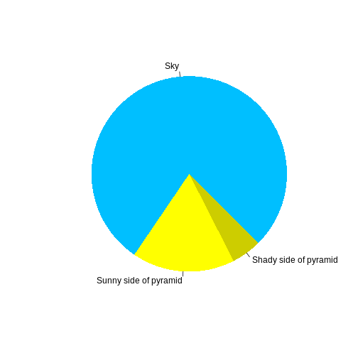
R
pie(
  c(Sky = 78, "Sunny side of pyramid" = 17, "Shady side of pyramid" = 5),
  init.angle = 315,
  col = c("deepskyblue", "yellow", "yellow3"),
  border = FALSE
)
Mermaid Diagrams
Mermaid
diagrams can be included in lessons by using the
mermaid fenced div and a code fragment the mermaid
syntax.
The following example creates a simple flowchart:
    flowchart LR
        accTitle: {A short figure title}
        accDescr: {A longer description of the figure, highlighting important elements}
        A(1. Step A)
        A --> B(2. Step B)
        C("`3. Step C
        - A thing
        - Another thing
        - Something else`")
        B --> C
        C --> D(4. Step D)
The resulting mermaid diagram will be rendered as:
    flowchart LR
        accTitle: {A short figure title}
        accDescr: {A longer description of the figure, highlighting important elements}
        A(1. Step A)
        A --> B(2. Step B)
        C("`3. Step C
        - A thing
        - Another thing
        - Something else`")
        B --> C
C --> D(4. Step D)Accessibility of Mermaid Diagrams
Note that both the accTitle and accDescr
fields in the mermaid code block need to be supplied to produce an
accessible figure caption!
accTitle provides a short title for the figure, and
accDescr provides a longer form description of the figure
that highlights important elements.
Both of these fields are read by screen readers to provide an accessible description of the figure.
Math
One of our episodes contains \(\LaTeX\) equations when describing how to create dynamic reports with {knitr}, so we now use mathjax to describe this:
$\alpha = \dfrac{1}{(1 - \beta)^2}$ becomes: \(\alpha = \dfrac{1}{(1 - \beta)^2}\)
Cool, right?
Glosario Terms
Glosario is the Carpentries data science glossary that is developed by the international community, providing terms, definitions and translations to make lessons more accessible.
{sandpaper} can automatically generate glossary links in lessons from links to Glosario terms in lesson content markdown.
Configuration
Firstly, to enable this behaviour, the glosario key
needs to be added to a lesson’s config.yaml.
For automatic retrieval of the latest glossary.yml from
Glosario’s GitHub repository, set:
For manual retrieval from a local (e.g. working on your lesson offline) or remote location (e.g. providing a specific Glosario version), supply a string relative/absolute path or URL to the config:
Lesson content
A lesson maintainer/contributor can add placeholders into the main content of lessons that sandpaper will subsequently process.
Sandpaper understands links to Glosario terms in two ways, either a template-style term, or a hard link to the term page, i.e.:
{{ glosario.<term> }}[<term>](https://glosario.carpentries.org/en/#<term>)
Automatic language selection
When using the template-style term, sandpaper will automatically
generate the URL link using the language specified in the
config.yaml lang setting.
When using the markdown link style, sandpaper will automatically
replace the en/ in the link with the language specified in
the config.yaml lang setting.
For example, if the config.yaml language is set to
lang: de:
[data_structure](https://glosario.carpentries.org/en/#data_structure)
will be replaced with:
[data_structure](https://glosario.carpentries.org/de/#data_structure)
If the term is not available in that language, a warning will be printed when the lesson builds, and it will default back to English.
Example output
To look at a specific example, the datacarpentry/spreadsheet-ecology-lesson can be edited to include Glosario links.
To add a glosario link to the term data structure at the
URL https://glosario.carpentries.org/en/#data_structure,
the markdown becomes:
The most common mistake made is treating spreadsheet programs like lab notebooks, that is, relying on context,
notes in the margin, spatial layout of data and fields to convey information. As humans, we can (usually) interpret
these things, but computers don't view information the same way, and unless we explain to the computer what
every single thing means (and that can be hard!), it will not be able to see how our data fits together. This is called
the data structure {{ glosario.data_structure }}.
Similarly, to add a link using the inline markdown link syntax, the markdown becomes:
Using the power of computers, we can manage and analyze data in much more effective and faster ways, but to
use that power, we have to set up our data for the computer to be able to understand it
(and computers are very [literal](https://glosario.carpentries.org/en/#literal)).
Once the lesson is built, this will produce the following output:
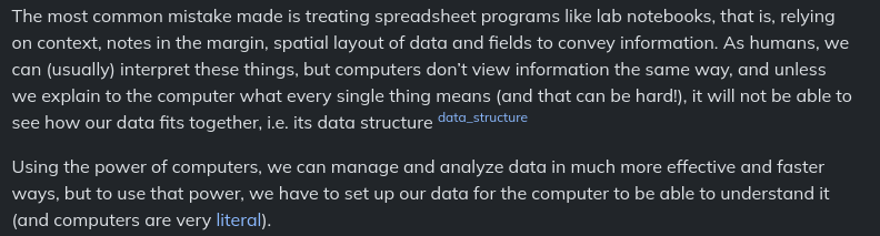
In the first example, {{ glosario.data_structure }} adds
a data_structure link as a superscript inline.
In the second example, a typical markdown link will be inserted.
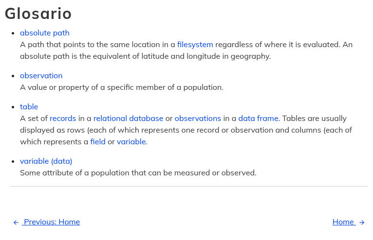
In either case, sandpaper will find these links and add them to the
global reference.md page in your lesson, built as
reference.html, and linked in the top lesson menu as
Glossary:
Unavailable terms
Users will receive a warning when using terms that are not in the currently selected config.yaml language for the lesson:
- Use
.Rmdfiles for lessons even if you don’t need to generate any code - Run
sandpaper::check_lesson()to identify any issues with your lesson - Run
sandpaper::build_lesson()to preview your lesson locally
The designation of “episode” will likely change. Throught UX testing, it’s clear that calling these lesson units “episodes” is confusing, even for people who have been in The Carpentries for several years. The current working proposal is to call these “chapters”.↩︎
Do not worry if you aren’t comfortable yet, that’s what we will show you in this episode!↩︎
Captions allow visually impaired users to choose if they want to skip over the table contents if it is scannable. For more information, you can read MDN docs: adding a caption to your table↩︎
Content from Editing a {sandpaper} lesson
Last updated on 2026-05-26 | Edit this page
Estimated time: 5 minutes
Overview
Questions
- What is the folder structure of a lesson?
- How do you download an existing {sandpaper} lesson?
Objectives
- Understand how to clone an existing lesson from GitHub
- Use
sandpaper::build_lesson()to preview a lesson - Update the configuration for a lesson
- Rearrange the order of episodes
If you want to edit and preview a full lesson using {sandpaper}, this is the episode for you. If you want to create a new lesson, head back to the episode for Creating a New Lesson. I believe it’s beneficial to experience editing a fully functional lesson, so you will edit THIS lesson. The first step is to fork and clone it from GitHub:
Fork and Clone a Lesson
If you are familiar with the process of forking and cloning, then you may fork and clone as you normally do. If you would like a reminder, here are the steps:
Think about a place on your computer where you want to work on your fork of the lesson (e.g.
~/Documents/Lessons/) and make sure that folder exists.Go to https://github.com/carpentries/sandpaper-docs/fork/ to fork the repository to your account
(recommended) When creating your fork, you should uncheck “Copy the
mainbranch only” checkbox.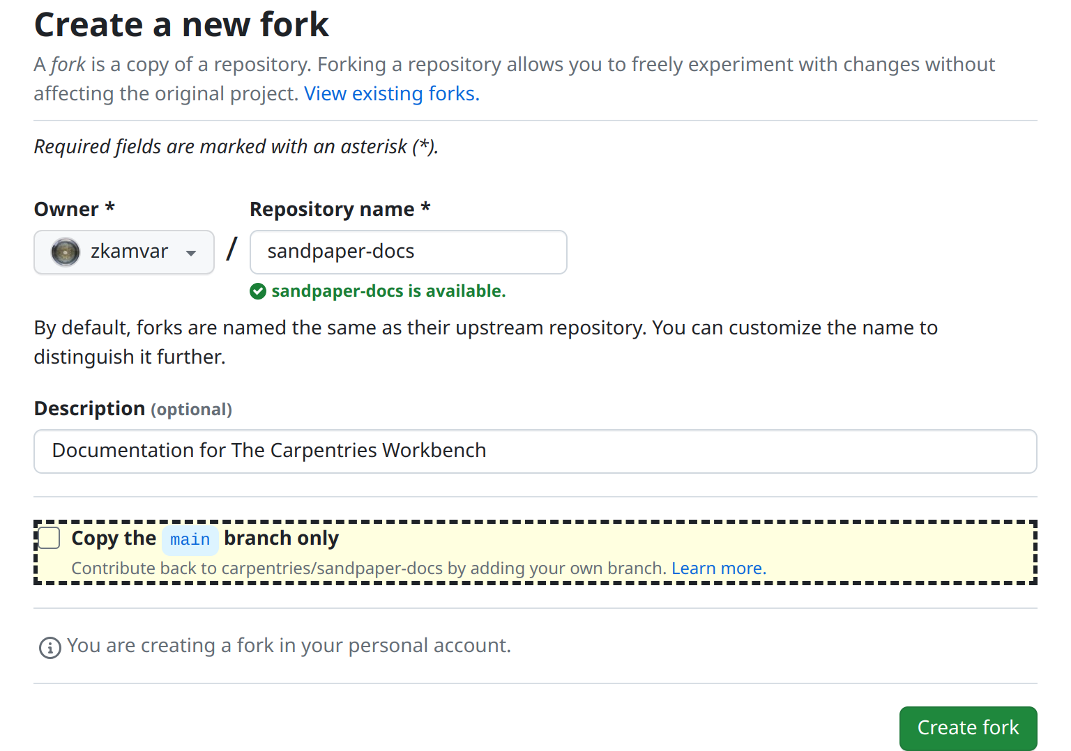
-
In the shell, use this command to clone this repository to your working directory, replacing
<USERNAME>with your username
One-step fork with R
If you use R and you also use an HTTPS protocol, you might be interested to know that the above three steps can be done in a single step with the {usethis} package via the GitHub API:
R
usethis::create_from_github("carpentries/sandpaper-docs", "~/Documents/Lessons/")
In the next section, we will explore the folder structure of a lesson.
Preview the Lesson
- Open the lesson in RStudio (or whatever you use for R)
- Use the keyboard shortcut ctrl + shift + b (cmd +
shift + b on macOS) to build and preview this lesson (or type
sandpaper::build_lesson()in the console if you are not using RStudio) - Open THIS file (
episodes/editing.md) and add step 4: preview the lesson again.
What do you notice?
What you should notice is that the only file updated when you
re-render the lesson is the file you changed
(episodes/editing.Rmd).
Folder Structure
🚧 This May Change 🚧
The exact folder structure still has the possibility to change based on user testing for the front-end of the lesson website.
The template folder structure will contain markdown files arranged so
that they match what we expect the menubar for the lesson should be. All
folders and files with an arrow <- are places in the
lesson template you will be modifying:
|-- .gitignore         #  | Ignore everything in the site/ folder
|-- .github/           #  | Configuration for deployment
|-- episodes/          # <- PUT YOUR EPISODE MARKDOWN FILES IN THIS FOLDER
|-- instructors/       # <- Information for Instructors (e.g. guide.md)
|-- learners/          # <- Information for Learners (e.g. reference.md and setup.md)
|-- profiles/          # <- Learner and/or Instructor Profiles
|-- site/              #  | This is a "scratch" folder ignored by git and is where the rendered markdown files and static site will live
|-- config.yaml        # <- Use this to configure lesson metadata
|-- index.md           # <- The landing page of your site
|-- CONTRIBUTING.md    #  | Carpentries Rules for Contributions (REQUIRED)
|-- CODE_OF_CONDUCT.md #  | Carpentries Code of Conduct (REQUIRED)
|-- LICENSE.md         #  | Carpentries Licenses (REQUIRED)
`-- README.md          # <- Introduces folks how to use this lesson and where they can find more information.
This folder structure is heavily opinionated towards achieving our goals of creating a lesson infrastructure that is fit for the purpose of delivering lesson content for not only Carpentries instructors, but also for learners and educators who are browsing the content after a workshop. It is not designed to be a blog or commerce website. Read the following sections to understand the files and folders you will interact with most.
All source files in {sandpaper} are written in pandoc-flavored markdown and all require
yaml header called title. Beyond that, you can put anything
in these markdown files.
config.yaml
This configuration file contains global information about the lesson. It is purposefully designed to only include information that is editable and relevant to the lesson itself and can be divided into two sections: information and organization
Information
These fields will be simple key-pair values of information used throughout the episode
- carpentry
- The code for the specific carpentry that the lesson belongs to (swc, dc, lc, cp, incubator, lab)
- carpentry_description
- (Optional) Full organisation name. Not needed when carpentry is swc, dc, lc, cp, incubator, or lab.
Adding a custom logo
The “carpentry” variable works with the {varnish} package to control the logo displayed on your lesson. You can display your own logo by
- Adding the logo file as SVG (e.g. ‘ice-cream-logo.svg’) to your fork
of {varnish} in the
inst/pkgdown/assets/assets/imagesfolder. - Setting “carpentry” to match the beginning of the name of your logo
file. E.g. to use the
ice-cream-logo.svgfile given above, “carpentry” should be set to ‘ice-cream’. - Adding ‘varnish: [YOUR-GITHUB-USERNAME]/varnish’ to the
Customization section of your lessons
config.yamlfile.
The rendered lesson will display your logo file with alternative text that matches the value of “carpentry”. For more informative alternative text, you can set “carpentry_description” to your organisation’s full name. E.g. “Ice Cream Carpentry” instead of “ice-cream”.
- title
- The main title of the lesson
- lang
-
Two letter code for the language used for headers, callouts and other
Workbench elements. Defaults to
enfor English. - languages
- If the lesson is available in more than one language you can use this setting to provide a drop-down menu to navigate between languages. This option can also be used to link between different flavors of the same material (e.g. Python vs R, GitHub vs GitLab)
Offering 4 languages: English, Spanish, German and Italian
An example to illustrate the usage of lang and
languages in a lesson config.yaml. The default
language is English and is indicated by the lang attribute.
The languages attribute specifies the names in the
drop-down menu and links to access the alternative content.
- Add
lang: ento indicate that the current lesson is in English - Indicate the
defaultlanguage to be English, shown as the default option in the drop-down. - Provide
otherlanguages, their description and a link to the corresponding location.
- life_cycle
- What life cycle is the lesson in? (pre-alpha, alpha, beta, stable)
- license
- The license the lesson is registered under (defaults to CC-BY 4.0)
Changing the default license
The default license for a lesson created with {sandpaper} is CC-BY 4.0. To use a different license
- Change the “license” variable to the name of your desired license.
- Replace the contents of ‘LICENSE.md’ with the text of your license or add a new variable called “license_url” and set to the url for your license.
- source
- The github source of the lesson
- branch
- The default branch
- contact
- Who should be contacted if there is a problem with the lesson
Organization
These fields match the folder names in the repository and the values
are a list of file names in the order they should be displayed. By
default, each of these fields is blank, indicating that the default
alphabetical order is used. To list items, add a new line with a hyphen
and a space preceding the item name (-). For example, if I
wanted to have the episodes called “one.md”, “two.Rmd”, “three.md”, and
“four.md” in numerical order, I would use:
Below are the four possible fields {sandpaper} will recognize:
- episodes
- The names of the episodes (main content)
- instructors
- Instructor-specific resources (e.g. outline, etc)
- learners
- Resources for learners (e.g. Glossary terms)
- profiles
- Learner profile pages
Remove Episode Numbering
By default, the lesson sidebar will display numbers next to each
episode title. To remove these numbers, add the following line to your
config.yaml file.
disable_sidebar_numbering: true
Configuring Episode Order
Open config.yaml and change the order of the episodes.
Preview the lesson after you save the file. How did the schedule
change?
The episodes appear in the same order as the configuration file and the timings have rearranged themselves to reflect that.
Configuring web analytics
The optional analytics field can be used to configure
web analytics, e.g. with Matomo or
Google Analytics. There are currently three options for
analytics:
-
NULL: disables tracking for that lesson. This is the default behviour, and is equivalent to omitting theanalyticsfield fromconfig.yamlaltogether. -
carpentries: adds the tracking script needed for the lesson to be tracked by The Carpentries self-hosted Matomo system. This option works only for The Carpentries lessons: community-owned lessons cannot be tracked in the same way. -
<user_string>: allows the user to define their own tracker script string. For legibility, use the|symbol to indicate that the value of the YAML field will be split across multiple indented lines (known as a ‘literal block’ in YAML). For example, to configure for Google Analytics:
YAML
analytics: |
  <!-- Global site tag (gtag.js) - Google Analytics -->
  <script async src='https://www.googletagmanager.com/gtag/js?id={YOUR TRACKING ID}#' ></script>
  <script>
    window.dataLayer = window.dataLayer || [];
    function gtag(){dataLayer.push(arguments);}
    gtag('js', new Date());

    gtag('config', '{YOUR TRACKING ID}');
  </script>
Tracking scripts configured with the analytics option
are added to the footer element of the lesson website HTML.
episodes/
This is the folder where all the action is. It contains all of the episodes, figures, and data files needed for the lesson. By default, it will contain an episode called introduction.Rmd. You can edit this file to use as your introduction. To create a new Markdown episode, use the folowing function:
R
sandpaper::create_episode_md("Episode Name")
This will create a Markdown episode called
episode-name.md in the episodes/ directory of
your lesson, pre-populated with objectives, questions, and keypoints.
The episode will be added to the end of the episodes: list
in config.yaml, which serves as the table of contents.
If you want to create an episode, but are not yet ready to render or
publish it, you can create a draft using the draft_episode
family of functions:
R
sandpaper::draft_episode_rmd("Visualising Data")
This will create an R Markdown episode called
visualising-data.Rmd in the episodes/
directory of your lesson, but it will NOT be added to
config.yaml, allowing you to work on it at your own pace
without the need to publish it.
When you are ready to publish an episode or want to move an existing
episode to a new place, you can use move_episode() to pull
up an interactive menu for moving the episode.
R
sandpaper::move_episode("visualising-data.Rmd")
OUTPUT
ℹ Select a number to insert your episode
(if an episode already occupies that position, it will be shifted down)

1. introduction.md
2. episode-name.md
3. [insert at end]

Choice: Should I use R Markdown or Markdown Episodes?
All {sandpaper} lessons can be built using Markdown, R Markdown, or a mix of both. If you want to dynamically render the output of your code via R (other languages will be supported in the future), then you should use R Markdown, but if you do not need to dynamically render output, you should stick with Markdown.
Sandpaper offers four functions that will help with episode creation depending on your usage:
| R Markdown | Markdown |
|---|---|
create_episode_rmd() |
create_episode_md() |
draft_episode_rmd() |
draft_episode_md() |
instructors/
This folder contains information used for instructors only. Downloads of code outlines, aggregated figures, and slides would live in this folder.
learners/
All the extras the learner would need, mostly a setup guide and glossary live here.
The glossary page is populated from the reference.md
file in this folder. The format of the glossary section of the
reference.md file is a heading title
## Glossary followed by a definition
list. Definition lists are formatted as two lines for each term, the
first includes the term to be defined and then the second line starts
with a “:” and a space then the definition. i.e.
- term
- definition
profiles/
Learner profiles would live in this folder and target learners, instructors, and maintainers alike to give a focus on the lesson.
index.md
This is the landing page for the lesson. The schedule is appended at the bottom of this page and this will be the first page that anyone sees.
README.md
This page gives information to maintainers about what to expect inside of the repository and how to contribute.
Making your lesson citable
You can add information about how people should cite your lesson by
adding a citation file to your lesson repository. If the root folder of
your lesson repository contains a CITATION.cff in Citation
File Format (more details below), the lesson website will include a
Lesson Citation page linked from Cite in the page footer. If
the root folder includes a file called CITATION, the
‘Cite’ page footer of your lesson site will link to this
file.
We recommend that you add and maintain a CITATION.cff
file for your lesson, in Citation File Format
(CFF). CFF is a structured text file format that provides
machine-readable citation information for projects. It is supported by a
growing number of tools, including GitHub: if a project includes a CFF
file in its default branch, GitHub
will present citation information for the project under a ‘Cite
this repository’ button in the About sidebar.
Creating a CFF for a lesson
You can use the cffinit
webtool to create a new CFF for your lesson or update an existing
file. When creating a CFF for a lesson, you should specify
dataset as the type of work being described (This
discussion includes explanation for why dataset is the
appropriate type for a lesson.)
cff-version: 1.2.0
title: Introduction to The Carpentries Workbench
message: >-
  Please cite this lesson using the information in this file
  when you refer to it in publications, and/or if you
  re-use, adapt, or expand on the content in your own
  training material. To cite the Workbench software itself,
  please refer to the websites for the individual
  components:
  https://carpentries.github.io/sandpaper/authors.html#citation,
  https://carpentries.github.io/pegboard/authors.html#citation,
  https://carpentries.github.io/varnish/authors.html#citation
type: dataset
authors:
  - given-names: Zhian
    family-names: Kamvar
    name-particle: N.
    orcid: 'https://orcid.org/0000-0003-1458-7108'
  - given-names: Toby
    family-names: Hodges
    email: tobyhodges@carpentries.org
    affiliation: The Carpentries
    orcid: 'https://orcid.org/0000-0003-1766-456X'
  - given-names: Erin
    family-names: Becker
    orcid: 'https://orcid.org/0000-0002-6832-0233'
  - orcid: 'https://orcid.org/0000-0002-7040-548X'
    given-names: Sarah
    family-names: Stevens
  - given-names: Michael
    family-names: Culshaw-Maurer
    orcid: 'https://orcid.org/0000-0003-2205-8679'
  - given-names: Maneesha
    family-names: Sane
  - given-names: Robert
    family-names: Davey
    orcid: 'https://orcid.org/0000-0002-5589-7754'
  - given-names: Amelia
    family-names: Bertozzi-Villa
  - given-names: Kaitlin
    family-names: Newson
    orcid: 'https://orcid.org/0000-0001-8739-5823'
  - given-names: Jennifer
    family-names: Stubbs
    orcid: 'https://orcid.org/0000-0002-6080-5703'
  - given-names: Belinda
    family-names: Weaver
  - given-names: François
    family-names: Michonneau
    orcid: 'https://orcid.org/0000-0002-9092-966X'
repository-code: 'https://github.com/carpentries/sandpaper-docs'
url: 'https://carpentries.github.io/sandpaper-docs/'
abstract: >-
  Documentation for The Carpentries Workbench, a set of
  tools that can be used to create accessible lesson
  websites.
keywords:
  - Carpentries
  - sandpaper
  - pegboard
  - varnish
  - R
  - pkgdown
license: CC-BY-4.0
Plain text CITATION file
As an alternative to Citation File Format, you can also use a plain
text file, named CITATION (i.e. without the
.cff extension), in which you add guidance for people
wanting to cite your lesson in their publications/projects.
Please cite this lesson as:

Zhian N. Kamvar et al,
Introduction to The Carpentries Workbench.
https://github.com/carpentries/sandpaper-docs-
sandpaper::build_lesson()renders the site and rebuilds any sources that have changed. - RStudio shortcuts are cmd + shift + B and cmd + shift + K
- To edit a lesson, you only need to know Markdown and/or R Markdown
- The folder structure is designed with maintainers in mind
- New episodes can be added with
sandpaper::create_episode()
Content from EXAMPLE: Using RMarkdown
Last updated on 2026-05-26 | Edit this page
Estimated time: 7 minutes
Overview
Questions
- How do you write a lesson using R Markdown and sandpaper?
Objectives
- Explain how to use markdown with the new lesson template
- Demonstrate how to include pieces of code, figures, and nested challenge blocks
Introduction
This is a lesson created via The Carpentries Workbench. It is written in Pandoc-flavored Markdown for static files and R Markdown for dynamic files that can render code into output. Please refer to the Introduction to The Carpentries Workbench for full documentation.
What you need to know is that there are three sections required for a valid Carpentries lesson template:
-
questionsare displayed at the beginning of the episode to prime the learner for the content. -
objectivesare the learning objectives for an episode displayed with the questions. -
keypointsare displayed at the end of the episode to reinforce the objectives.
Inline instructor notes can help inform instructors of timing challenges associated with the lessons. They appear in the “Instructor View”
Code fences
Code fences written in standard markdown format will be highlighted, but not evaluated:
Code fences written using R Markdown chunk notation will be highlighted and executed:
R
magic <- sprintf("47 plus 2 equals %d\n47 times 2 equals %d", 47 + 2, 47 * 2)
cat(magic)
OUTPUT
47 plus 2 equals 49
47 times 2 equals 94
It’s magic!
Challenge 1: Can you do it?
What is the output of this command?
R
paste("This", "new", "lesson", "looks", "good")
OUTPUT
[1] "This new lesson looks good"Challenge 2: how do you nest solutions within challenge blocks?
You can add a line with at least three colons and a
solution tag.
Figures
You can also include figures generated from R Markdown:
R
pie(
  c(Sky = 78, "Sunny side of pyramid" = 17, "Shady side of pyramid" = 5),
  init.angle = 315,
  col = c("deepskyblue", "yellow", "yellow3"),
  border = FALSE
)

Or you can use standard markdown for static figures with the following syntax:
{alt='alt text for accessibility purposes'}
For example:
{alt='Blue Carpentries hex person logo with no text.'}
Additional
attributes can be specified for the image alongside the alternative
text description in the {}. Some, like width
and height, can be specified directly:
{alt='Blue Carpentries hex person logo with no text.' width='25%'}
🎨 Advanced Image Styling
More complex styling with arbitrary CSS is also possible within the
Workbench, by providing CSS directives (separated by ;) to
a style attribute inside the {}.
However, you should be aware that all styling must be described
in this style attribute if it is present,
i.e. width and height must be included as CSS
directives within the style attribute when it is
used.
For example, to introduce some padding around the resized image:
{alt='Blue Carpentries hex person logo with no text.' style='padding:10px; width:25%'}
Note the use of : for the key-value pairs of CSS
directives defined within style.
Math
One of our episodes contains \(\LaTeX\) equations when describing how to create dynamic reports with {knitr}, so we now use mathjax to describe this:
$\alpha = \dfrac{1}{(1 - \beta)^2}$ becomes: \(\alpha = \dfrac{1}{(1 - \beta)^2}\)
Cool, right?
- Use
.mdfiles for episodes when you want static content - Use
.Rmdfiles for episodes when you need to generate output - Run
sandpaper::check_lesson()to identify any issues with your lesson - Run
sandpaper::build_lesson()to preview your lesson locally
Content from Lesson Deployment
Last updated on 2026-05-26 | Edit this page
Estimated time: 5 minutes
Overview
Questions
- What is the two-step model of deployment?
- Why do we preserve both generated markdown and HTML?
Objectives
- Understand the two-step model for lesson deployment
- Understand how our lessons are deployed on GitHub
Building A Lesson
Static site generators all know one thing: how to translate markdown to an HTML website. The Carpentries Lesson Infrastructure is no different in that it will generate an HTML website from markdown files using pandoc. The difference is how we handle the generated content to make your lesson portable and transferrable.
Working With Generated Content
The Carpentries has formally supported generated content from R lessons in the form of R Markdown files since 2016 and we are working on a solution to incorporate generated content from other languages in the future. If you do not use generated content in your lesson, you can skip this section.
The default paradigm for R Markdown is to first generate markdown output from the R Markdown document, convert it to HTML, and then discard the generated markdown output.

However, this default behavior for generated content is not conducive for collaboration on lessons because the outputs often live in the same place as the source files. Moreover, if any changes occur in the software used to generate content, inspecting the differences between two HTML files is difficult because of markup. We created the {sandpaper} package to alleviate these downsides by clearly separating the generated content from the source material by taking advantage of a two-step model of deployment.
The Two-Step Model of Deployment
To alleviate the downsides of working with generated content, The
Carpentries Workbench employs a two-step model of deployment when you
run sandpaper::build_lesson()
- Take any source files with content that needs to be interpreted (e.g. R Markdown) and render them to markdown in a staging area ignored by git.
- Apply the HTML style to the markdown files in the staging area to create the lesson website.

All of the generated content lives in the site/ folder,
and importantly: it is all cached and ignored by git. Ignoring generated
content locally means that the source of truth for these files is no
longer dependent on the maintainer’s local setup.
The reason we have this model is also for portability. It’s because markdown output is a lot easier to audit than HTML when something goes wrong, rendered markdown can be transferred to other contexts (e.g. books or blogposts), and we can swap out the generators without needing to rewrite the entire pipeline.
Did you know?
When the lesson is pushed to GitHub, all of the generated content IS stored in separate branches so that we can provide a way for you to audit changes from pull requests.
Deploying On GitHub
For historical reasons, GitHub used the Jekyll static site generator to deploy their documentation websites, but because we no longer use Jekyll, we we deploy our sites in a different manner.
On GitHub, we store generated content in two orphan branches called
md-outputs and gh-pages for the generated
markdown and html, respectively. We use GitHub Actions Workflows
to build, validate, and deploy our lessons on GitHub pages. Because the
markdown and HTML outputs are preserved in the git history, we can tag
and preserve them for archiving.
These workflows are the source of truth for the lessons and will keep your lesson up-to-date with the latest version of the HTML template. Moreover, each week, these workflows will check for updates and, if there are any, a pull request will be created to ensure you are using the latest versions. You can read more about updating your workflows in the Maintenance chapter.
If you use R Markdown in your lesson, you will notice that for every
pull request (PR), a GitHub bot comments on your pull requests informing
you about what content has changed and gives you a link to the
differences between the current state of the md-outputs
branch and the proposed changes. You can find out more about this in the
Pull Request chapter.
- Lessons are built using a two-step process of caching markdown outputs and then building HTML from that cache
- We use GitHub Actions to deploy and audit generated lesson content to their websites
Content from Maintaining a Healthy Infrastructure
Last updated on 2026-05-26 | Edit this page
Estimated time: 12 minutes
Overview
Questions
- What are the four components of the lesson infrastructure?
- What lesson components are auto-updated on GitHub?
Objectives
- Identify components of the workbench needed for lesson structure, validation, styling, and deployment
- Understand how to update R packages
- Understand how to update GitHub workflows
🚧 Under Development
This episode is still actively being developed
Introduction
The Carpentries Lesson Infrastructure is designed to be cu
Maintainer Tools
This is {sandpaper}! It takes your source files and generates the outputs!
Update in R with:
R
install.packages("sandpaper", repos = "https://carpentries.r-universe.dev")
Validator
This is {pegboard}! It runs behind the scenes in {sandpaper} to parse the source documents and validate things like headings, images, and cross-links. It also can extract elements like code and individual sections.
Update in R with:
R
install.packages("pegboard", repos = "https://carpentries.r-universe.dev")
Styling
This is {varnish}! This package contains all the HTML, JavaScript, and CSS to make your generated HTML look like a Carpentries Lesson!
Update in R with:
R
sandpaper::update_varnish()
Deployment
Updating Your Deployment Workflows
The workflows are the the only place in our lesson that needs to be kept up-to-date with upstream changes from {sandpaper}. While we try as much as possible to keep the functionality of {sandpaper} inside the package itself, there are times when we need to update the GitHub workflows for security or performance reasons. You can update your workflows in one of two ways: via GitHub or via {sandpaper}.
🚧 Under Development
Workflow updates are still underdevelopment, but are
available for use. We are exploring different methods for
making these unobtrusive as possible such as specifying scheduled
updates via config.yaml and even creating a bot that will
remove the need for this workflow.
On Schedule (default)
The workflow update workflow is scheduled to run every Tuesday at 00:00 UTC. If there are any changes in the upstream workflows, then a Pull Request will be created with the new changes. If there are no changes to the workflows, then the process will silently exit and you will not be notified.
Via GitHub
To update your workflows in GitHub, go to
https://github.com/(ORGANISATION)/(REPOSITORY)/actions/workflows/update-workflows.yaml
Once there, you will see a button that says “Run Workflow” in a blue field to the right of your screen. Click on that Button and it will give you two options:
- “Who this build (enter github username to tag yourself)?
- “Workflow files/file extensions to clean (no wildcards, enter”” for none)
You can leave these as-is or replace them with your own values. You can now hit the green “Run Workflow” button at the bottom.
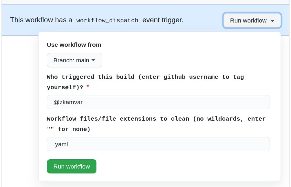
After ~10 seconds, your workflow will run and a pull request will be created from a GitHub bot (at the moment, this is @znk-machine) if your workflows are in need of updating.
Check the changes and merge if they look okay to you. If they do not, contact @tobyhodges.
Via R
If you want to update your workflows via R, you can use the
update_github_workflows() function, which will report which
files were updated.
R
sandpaper::update_github_workflows()
OUTPUT
ℹ Workflows/files updated:
- .github/workflows/pr-comment.yaml (modified)
- .github/workflows/pr-post-remove-branch.yaml (modified)
- .github/workflows/README.md (modified)
- .github/workflows/sandpaper-version.txt (modified)
- .github/workflows/update-workflows.yaml (new)
After that, you can add and commit your changes and then push them to GitHub.
Do not combine workflow changes with other changes
If you bundle a workflow changes in a pull request, you will not get the benefit of being able to inspect the output of the generated markdown files. Moreover, while we try to make these workflow files as simple as possible, they are still complex and would distract from any content that would be proposed for the lesson.
- Lesson structure, validation, and styling components are all updated automatically on GitHub.
- Lesson structure, validation, and styling components all live in your local R library.
- Locally, R packages can be updated with
install.packages() - Package styling can be updated any time with
sandpaper::update_varnish() - GitHub workflows live inside the lesson under
.github/workflows/ - GitHub workflows can be updated with
sandpaper::update_github_workflows()
Content from Auditing Pull Requests
Last updated on 2026-05-26 | Edit this page
Estimated time: 5 minutes
Overview
Questions
- What happens during a pull request?
- How do I review generated content of a pull request?
- How do I handle a pull request from a bot?
Objectives
- Identify key features of a pull request to review
- Identify the benefits of pull request comments from a bot
- Understand why bots will initiate pull requests
- Understand the purpose of automated pull requests
Introduction
One of the biggest benefits of working on a Carpentries Lesson is that it gives maintainers and contributors practice collaboratively working on GitHub and practicing common software engineering practices, including pull requests and reviews. In the Carpentries Workbench, we have implemented new features that will make reviewing contributed content easier for maintainers:
- Source content is checked for valid headings, links, and images
- Generated content is rendered to markdown and placed in a temporary branch for visual inspection.
- Pull requests are checked for malicious attacks.
Reviewing A Pull Request
When you recieve a pull request, a check will first validate that the lesson can be built and then, if the lesson can be built, it will generate output and leave a comment that provides information about the rendered output:
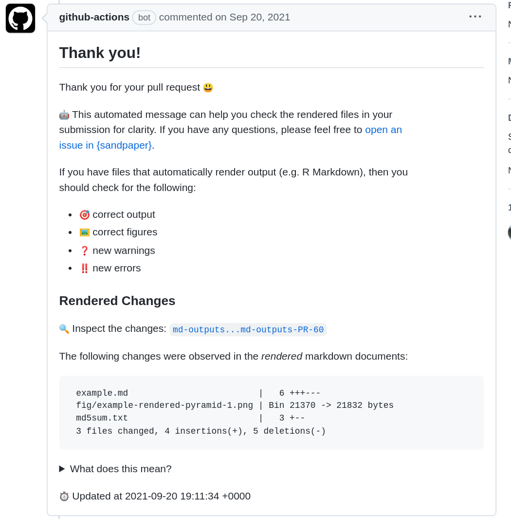
With this information, you can click on the link that says ‘Inspect the changes’ to navigate to a diff of the rendered files. In this example, we have manipulated the output of a plot, and GitHub allows us to visually inspect these differences by scrolling down to the file mentioned in the diff and clicking on the “file” icon to the top right, which indicates to “display the rich diff”.
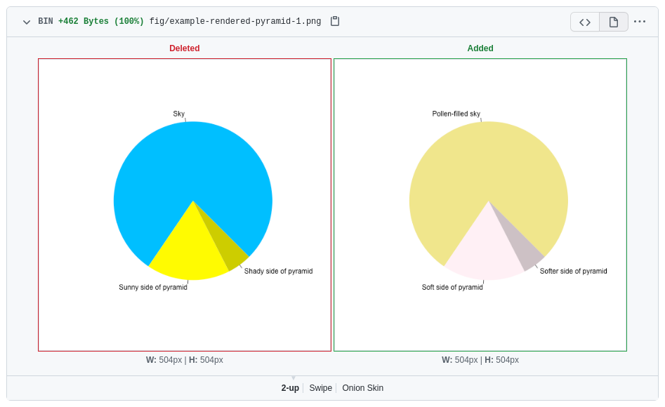
Living with Entropy
In R Markdown documents, If you use any sort of code that generates
random numbers, you may end up with small changes that show up on the
list of changed files. See this example where using
the ggplot2 function geom_jitter() leads to
slightly different image files. You can fix this by setting a seed
for the random number generator (e.g. set.seed(1)) at the
beginning of the episode, so that the same random numbers are generated
each time the lesson is built.
Of course, if you have a rendered lesson, another important thing is to check to make sure the outputs continue to work. If you notice any new errors or warnings new in the diff, you can work with the contributor to resolve them.
Risk Management
Accepting generated content into lessons from anyone runs the risk of a security breach by exposing secrets. To mitigate this risk, GitHub limits the scope of what is possible inside a pull request so that we can check and render the content without risk of exploitation. Through this, we render and check the lesson inside the pull request with no privileges, check that the pull request is valid (not malicious), and then create a temporary branch for an exploratory preview, allowing the maintainer to audit the generated content before it gets adopted into the curriculum.
If the PR is invalid (e.g. the contributor spoofed a separate, valid PR, or modified one of the github actions files), then the maintainer is alerted that the PR is potentially risky (see the Being Vigilant section for details)

Automated Pull Requests
There are two situations where you would receive a pull request from The Carpentries Apprentice bot
- The workflows need to be updated to the latest versions
- You have a lesson that uses generated content, the software requirements file (e.g. renv.lock or [future] requirements.txt) is updated to the latest versions and the lesson is re-built.
More details about the purpose of these builds can be found in The Chapter on updating lesson components.
For Lessons Outside of The Carpentries
If you are using {sandpaper} to work on a lesson on your own personal account, these pull requests may never trigger. If you want them to work, follow the instructions in the technical article in {sandpaper} called [Working with Automated Pull Requests].
Workflow Updates
When you receive a workflow update pull request, it will be on a
branch called update/workflows, state that it is a bot and
then indicate which version of sandpaper the workflows will be updated
to.
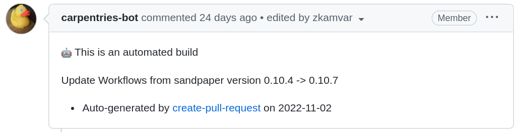
Because this PR contains changed workflow files, it will be marked as invalid no preview will be created, rendering a comment that indicates as such.
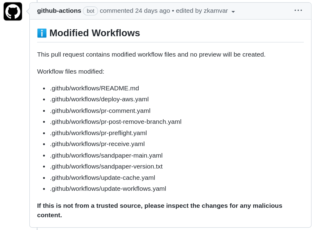
Updating Package Cache
Updates to the package cache are on the updates/packages
branch and accompanied by a bot comment that indicates the package
versions that have been updated.
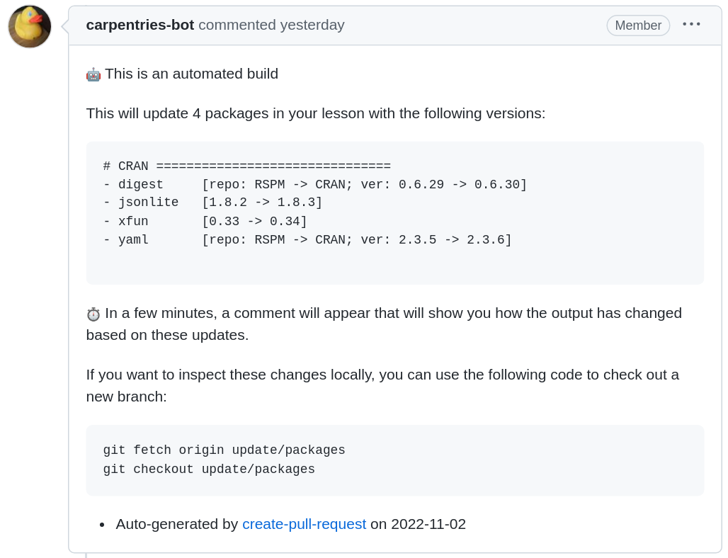
You will notice at the bottom of the comment there are instructions for how to check out a new branch and inspect the changes locally:
You are free to push code changes to this branch to update any lesson material that has changed due to package updates or you can also pin the versions of the packages you do not want updated.
Status Updates
When the pull request comes in from [The Carpentries Apprentice], you will see this comment immediately:
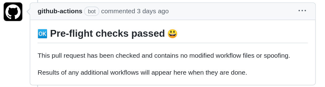
In the next couple of minutes, the R Markdown files will be re-built with the updated versions of the packages and the comment will update to reveal changes that have been made (if any).
Being Vigilant
Preventing Malicious Commits
The pull request previews are designed to allow you to inspect the potential changes before they go live. Because our lessons run arbitrary code, it is important to inspect the changes to make sure that someone is not trying to insert anything malicious into your lesson. A good rule of thumb for maintaining your lesson is that if there are changes are changes you do not understand coming from someone other than @carpentries-bot, then, it’s a good idea to wait to merge until you can fully understand the changes that are being proposed.
One risk that might happen is if someone updates lesson content and the github workflows at the same time. If this happens, you will see a comment from the workflows that looks like this:
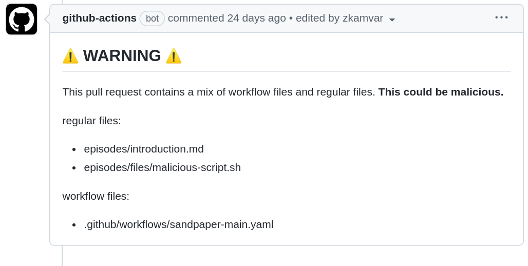
It is not always the case that changes in lesson files and workflow files will be bad, but it is not good practice to mix them.
Transition from carpentries/styles
During the migration to The Carpentries Workbench, we are using the lesson transition tool to convert lessons from the former “lesson template” to The Workbench. This involved removing commits unrelated to lesson content from the git history, which reduces the size of the lesson’s git repository and has the benefit of making the contribution log more clear. The downside is that forks that were created before the lesson was transferred to The Workbench suddenly became invalid.
If someone attempts to merge a pull request from an old repository, the first thing you will notice is hundreds of new commits and the second thing you will notice is the results of the automated check
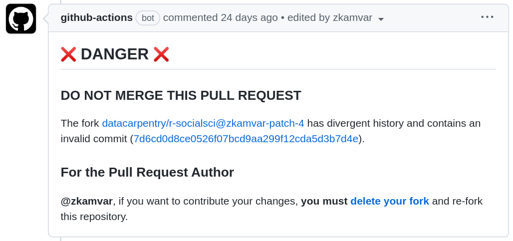
- Pull requests for generated formats requires validate of prose and generated content
- Inspecting the rendered markdown output can help maintainers identify changes that occur due to software before they are deployed to the website
- Automated pull requests help keep the infrastructure up-to-date