EXAMPLE: Using RMarkdown

Estimated time: 7 minutes

Overview

Questions

• How do you write a lesson using R Markdown and sandpaper?

Objectives

• Explain how to use markdown with the new lesson template
• Demonstrate how to include pieces of code, figures, and nested challenge blocks

Introduction

---

This is a lesson created via The Carpentries Workbench. It is written in Pandoc-flavored Markdown for static files and R Markdown for dynamic files that can render code into output. Please refer to the Introduction to The Carpentries Workbench for full documentation.

What you need to know is that there are three sections required for a valid Carpentries lesson template:

1. questions are displayed at the beginning of the episode to prime the learner for the content.
2. objectives are the learning objectives for an episode displayed with the questions.
3. keypoints are displayed at the end of the episode to reinforce the objectives.

Instructor Note

Inline instructor notes can help inform instructors of timing challenges associated with the lessons. They appear in the “Instructor View”

Code fences

Code fences written in standard markdown format will be highlighted, but not evaluated:

BASH

echo '47 + 2' | bc
echo '47 * 2' | bc

Code fences written using R Markdown chunk notation will be highlighted and executed:

R

magic <- sprintf("47 plus 2 equals %d\n47 times 2 equals %d", 47 + 2, 47 * 2) 
cat(magic)

OUTPUT

47 plus 2 equals 49
47 times 2 equals 94

It’s magic!

Challenge 1: Can you do it?

What is the output of this command?

R

paste("This", "new", "lesson", "looks", "good")

Output

OUTPUT

[1] "This new lesson looks good"

Challenge 2: how do you nest solutions within challenge blocks?

Show me the solution

You can add a line with at least three colons and a solution tag.

Figures

---

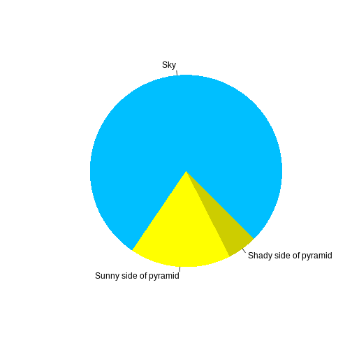
You can also include figures generated from R Markdown:

R

pie(
  c(Sky = 78, "Sunny side of pyramid" = 17, "Shady side of pyramid" = 5), 
  init.angle = 315, 
  col = c("deepskyblue", "yellow", "yellow3"), 
  border = FALSE
)

Sun arise each and every morning

Or you can use standard markdown for static figures with the following syntax:

![optional caption that appears below the figure](figure url){alt='alt text for accessibility purposes'}

For example:

![You belong in The Carpentries!](fig/Badge_Carpentries.svg){alt='Blue Carpentries hex person logo with no text.'}

You belong in The Carpentries!

Additional attributes can be specified for the image alongside the alternative text description in the {}. Some, like width and height, can be specified directly:

![You belong in The Carpentries!](fig/Badge_Carpentries.svg){alt='Blue Carpentries hex person logo with no text.' width='25%'}

You belong in The Carpentries!

🎨Advanced Image Styling

More complex styling with arbitrary CSS is also possible within the Workbench, by providing CSS directives (separated by ;) to a style attribute inside the {}.

However, you should be aware that all styling must be described in this style attribute if it is present, i.e. width and height must be included as CSS directives within the style attribute when it is used.

For example, to introduce some padding around the resized image:

![You belong in The Carpentries!](fig/Badge_Carpentries.svg){alt='Blue Carpentries hex person logo with no text.' style='padding:10px; width:25%'}

You belong in The Carpentries!

Note the use of : for the key-value pairs of CSS directives defined within style.

Math

---

One of our episodes contains \(\LaTeX\) equations when describing how to create dynamic reports with {knitr}, so we now use mathjax to describe this:

$\alpha = \dfrac{1}{(1 - \beta)^2}$ becomes: \(\alpha = \dfrac{1}{(1 - \beta)^2}\)

Cool, right?

Key Points

• Use .md files for episodes when you want static content
• Use .Rmd files for episodes when you need to generate output
• Run sandpaper::check_lesson() to identify any issues with your lesson
• Run sandpaper::build_lesson() to preview your lesson locally